Gradient Trader Part 1: The Surprising Usefulness of Autoencoders
Using Autoencoders to Learn Most Salient Features from Time Series
This post is about a simple tool in deep learning toolbox: Autoencoder. It can be applied to multi-dimensional financial time series.
Autoencoder
Autoencoding is the practice of copying input to output or learning the identity function. It has an internal state called latent space \(h\) which is used to represent the input. Usually, this dimension is chosen to be smaller than the input(called undercomplete). Autoencoder is composed of two parts: an encoder \(f :{\mathcal {X}}\rightarrow {\mathcal {H}}\) and a decoder \(g :{\mathcal {H}}\rightarrow {\mathcal {Y}}\).
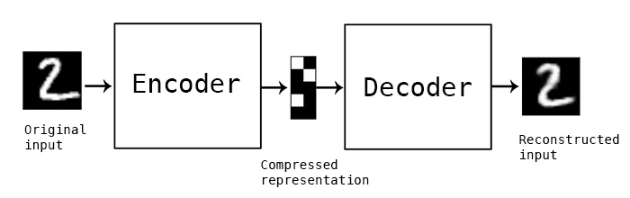
The hidden dimension should be smaller than \(x\), the input dimension. This way, \(h\) is forced to take on useful properties and most salient features of the input space.
Train an autoencoder to find function \(f, g\) such that:
\[\arg \min _{f, g}||X-(g \circ f )X||^{2}\]Recurrent Autoencoder
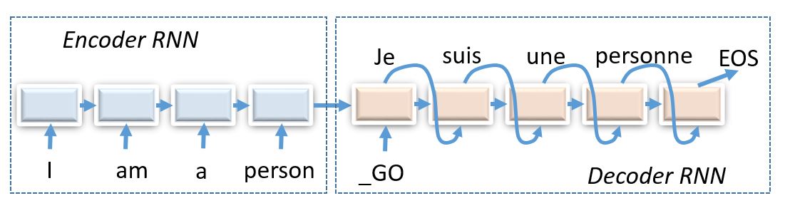
For time series data, recurrent autoencoder are especially useful. The only difference is that the encoder and decoder are replaced by RNNs such as LSTMs. Think of RNN as a for loop over time step so the state is kept. It can be unrolled into a feedforward network.
First, the input is encoded into an undercomplete latent vector \(h\) which is then decoded by the decoder. Recurrent autoencoder is a special case of sequence-to-sequence(seq2seq) architecture which is extremely powerful in neural machine translation where the neural network maps one language sequence to another.
import tensorflow as tf
import numpy as np
import matplotlib.pyplot as plt
Task
Copy a tensor of two sine functions that are initialized out of phase.
The shape of the input is a tensor of shape \((batch\_size, time\_step, input\_dim)\).
\(batch\_size\) is the number of batches for training. Looping over each sample is slower than applying a tensor operation on a batch of several samples.
\(time\_step\) is the number of timeframes for the RNN to iterate over. In this tutorial it is 10 because 10 points are generated.
\(input\_dim\) is the number of data points at each timestep. Here we have 2 functions, so this number is 2.
To deal with financial data, simply replace the \(input\_dim\) axis with desired data points.
- Bid, Ask, Spread, Volume, RSI. For this setup, the \(input\_dim\) would be 5.
- Order book levels. We can rebin the order book along tick axis so each tick aggregates more liquidity. An example would be 10 levels that are 1 stdev apart. Then \(input\_dim\) would be 10.
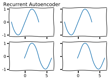
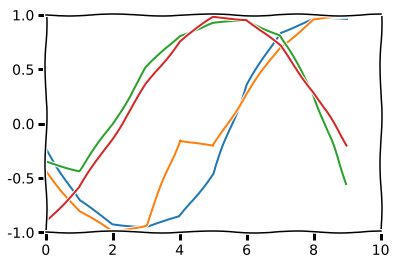
Here is an artist’s rendition of a recurrent autoencoder.
plt.xkcd()

x1 = np.linspace(-np.pi, np.pi)
y1 = np.sin(x1)
phi = 3
x2 = np.linspace(-np.pi+phi, np.pi+phi)
y2 = np.sin(x2)

f, ((ax1, ax2), (ax3, ax4)) = plt.subplots(2, 2, sharex=True, sharey=True)
ax1.plot(x1, y1)
ax1.set_title('Recurrent Autoencoder')
ax2.plot(x1, y1)
ax3.plot(x2, y2)
ax4.plot(x2, y2)
plt.show()
Generator
For each batch, generate 2 sine functions, each with 10 datapoints. The phase of the sine function is random.
import random
def gen(batch_size):
    seq_length = 10

    batch_x = []
    batch_y = []
    for _ in range(batch_size):
        rand = random.random() * 2 * np.pi

        sig1 = np.sin(np.linspace(0.0 * np.pi + rand,
                                  3.0 * np.pi + rand, seq_length * 2))
        sig2 = np.cos(np.linspace(0.0 * np.pi + rand,
                                  3.0 * np.pi + rand, seq_length * 2))
        x1 = sig1[:seq_length]
        y1 = sig1[seq_length:]
        x2 = sig2[:seq_length]
        y2 = sig2[seq_length:]

        x_ = np.array([x1, x2])
        y_ = np.array([y1, y2])
        x_, y_ = x_.T, y_.T

        batch_x.append(x_)
        batch_y.append(y_)

    batch_x = np.array(batch_x)
    batch_y = np.array(batch_y)

    return batch_x, batch_x#batch_y
Model
The goal is to use two numbers to represent the sine functions. Normally, we use \(\phi \in \mathbb{R}\) to represent the phase angle for a trignometric function. Let’s see if the neural network can learn this phase angle. The big picture here is to compress the input sine functions into two numbers and then decode them back.
Define the architecture and let the neural network do its trick. It is a model with 3 layers, a LSTM encoder that “encodes” the input time series into a fixed length vector(in this case 2). A RepeatVector that repeats the fixed length vector to 10 timesteps to be used as input to the LSTM decoder. For the decoder, we can either initialize the hidden state(memory) with the latent vector and use output at time \(t-1\) as input for time \(t\) or we can use latent vector \(h\) as the input at each timestep. These are called conditional and unconditional decoders.
from keras.models import Sequential, Model
from keras.layers import LSTM, RepeatVector

batch_size = 100
X_train, _ = gen(batch_size)

m = Sequential()
m.add(LSTM(2, input_shape=(10, 2)))
m.add(RepeatVector(10))
m.add(LSTM(2, return_sequences=True))
print m.summary()
m.compile(loss='mse', optimizer='adam')
history = m.fit(X_train, X_train, nb_epoch=2000, batch_size=100)
Epoch 1/2000
100/100 [==============================] - 0s - loss: 0.4845
Epoch 2000/2000
100/100 [==============================] - 0s - loss: 0.0280
m.summary()
_________________________________________________________________
Layer (type)                 Output Shape              Param #
=================================================================
lstm_37 (LSTM)               (None, 2)                 40
_________________________________________________________________
repeat_vector_12 (RepeatVect (None, 10, 2)             0
_________________________________________________________________
lstm_38 (LSTM)               (None, 10, 2)             40
=================================================================
Total params: 80
Trainable params: 80
Non-trainable params: 0
_________________________________________________________________
Since this post is a demonstration of the technique, we use the smallest model possible which happens to be the best in this case. The “best” dimensionality will be one that results in the highest lossless compression. In practice, it’s mostly an art than science. In production, there are a plethora of trick to accelerate training and finding the right capacity of the latent vector. Topics include: architectures for dealing with asynchronus, non-stationary time series, preprocessing techniques such as wavelet transforms and FFT.
plt.plot(history.history['loss'])
plt.ylabel("loss")
plt.xlabel("epoch")
plt.show()
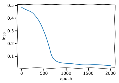
You may think that the neural network suddenly “got it” during training but this is just the optimzer escaping a saddle point. In fact, as we demonstrate below, the neural network(at least the decoder) doesn’t learn the math behind it at all.
X_test, _ = gen(1)
decoded_imgs = m.predict(X_test)

for i in range(2):
    plt.plot(range(10), decoded_imgs[0, :, i])
    plt.plot(range(10), X_test[0, :, i])
plt.title(dos_numeros)
plt.show()
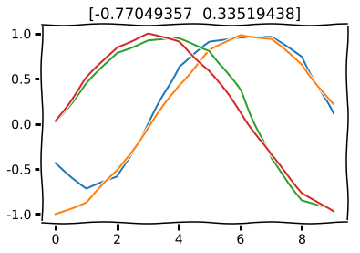
With more training, it would be even closer to input but that is not necessary for this demonstration.
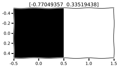
Visualize the latent vector can be useful sometimes but not in this case.
encoder = Model(m.layers[0].input, m.layers[0].output)
encoded_imgs = encoder.predict(X_test)
for i in range(len(encoded_imgs)):
    plt.imshow(encoded_imgs[i].reshape((1, 2)))
    plt.gray()
plt.title(encoded_imgs[i])
dos_numeros = encoded_imgs[i]
plt.show()
m.save('m.h5')
encoder.save('enc.h5')
decoder.save('dec.h5')
Visualization
The model successfully compressed 20 points to 2 points. It learned the most salient features from data. However in this case, the model is useless in that it has successfully learned \(g(f(x)) = x\) everywhere. Autoencoder are designed to copy imperfectly. Like all neural networks, autoencoders exploit the idea that data concentrates around a lower-dimensional manifold or a set of manifolds. The goal is to learn a function that behaves correctly on the data points from this manifold and exhibit unusual behavior everywhere off this manifold. In this case, we found a 2-D manifold tangent to the 20-D space. Here we discuss some visualization techniques.
Below we demonstrate what the manifold looks like when it is projected back to 20D with an animation. Ideally this shows how the decoder works.
x = Input(shape=(2,))
decoded = m.layers[1](x)
decoded = m.layers[2](decoded)
decoder = Model(x, decoded)
import matplotlib.animation as animation
from IPython.display import HTML
from numpy import random
fig, ax = plt.subplots()

x = range(10)

arr = decoder.predict(np.array([[-3.3, 0]]))
linea, = ax.plot(x, arr[0, :, 0])
lineb, = ax.plot(x, arr[0, :, 1])
ax.set_ylim(-1, 1)
ax.set_xlim(-0.1, 10.1)

def animate(i):
    ax.set_title("{0:.2f}, 0".format(-3.3+i/30.))
    arr = decoder.predict(np.array([[-3.3+i/30., 0]]))
    linea.set_ydata(arr[0, :, 0])
    lineb.set_ydata(arr[0, :, 1])
    return line,


# Init only required for blitting to give a clean slate.
def init():
    line.set_ydata(np.ma.array(x, mask=True))
    return line,

ani = animation.FuncAnimation(fig, animate, np.arange(1, 200), init_func=init,
                              interval=25, blit=True)
HTML(ani.to_html5_video())
fig, ax = plt.subplots()

x = range(10)

arr = decoder.predict(np.array([[-3.3, -3.3]]))
linea, = ax.plot(x, arr[0, :, 0])
lineb, = ax.plot(x, arr[0, :, 1])
ax.set_ylim(-1, 1)
ax.set_xlim(-0.1, 10.1)

def animate(i):
    ax.set_title("{0:.2f}, {0:.2f}".format(-3.3+i/30.))
    arr = decoder.predict(np.array([[-3.3+i/30., -3.3+i/30.]]))
    linea.set_ydata(arr[0, :, 0])
    lineb.set_ydata(arr[0, :, 1])
    return line,


# Init only required for blitting to give a clean slate.
def init():
    line.set_ydata(np.ma.array(x, mask=True))
    return line,

ani = animation.FuncAnimation(fig, animate, np.arange(1, 200), init_func=init,
                              interval=25, blit=True)
HTML(ani.to_html5_video())
As we can see from the animation above. The neural network is not using phase angle as the latent space. Instead, it is using a complex interaction between these two numbers caused by the gradient of LSTM during the training process. As \(x \rightarrow \infty\), the decoder \(g(h) \rightarrow 0\). This is understood as the decoder does not learn the underlying trig function but merely approximated a manifold of the high dimensional space.
Now let us visualize the latent space in its entirety. For higher dimensional latent space we may encounter in financial data, we can use PCA and tSNE but these are beyond the scope of this post.
X_test, _ = gen(1000)
latent_vec = encoder.predict(X_test)
plt.scatter(latent_vec[:, 0], latent_vec[:, 1])
plt.xlim(-1,1)
plt.ylim(-1,1)
plt.show()
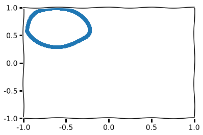
This circle you see above is the image under the encoder \(f(x)\) in the latent space \(H\). As you may have guessed from the beginning, since the trig map projects cartesian coordinate to a polar coordinate. The encoded vector is a linear subspace. A circle in polar coordinate has the equation \(r = a\). I hope this is a good enough punchline for those who didn’t hypothesize this result.
With PCA, any high-dimensional space can be projected into several linear subspaces using the Gram-Schmidt algorithm in linear algebra.
Anomaly Detection
As you can see, autoencoding is an extremely powerful technique in data visualization and exploration. But there are more depth to autoencoding besides creating pretty graphs. One application is anomaly detection.
Regulators can identify illegal trading strategies by building an unsupervised deep learning algorithm.
In data mining, anomaly detection (or outlier detection) is the identification of observations that do not conform to an expected pattern in a dataset. The ability to train a neural network in unsupervised manner allows autoencoders to shine in this area. Auto encoders provide a very powerful alternative to traditional methods for signal reconstruction and anomaly detection in time series.
Training an autoencoder is conceptually simple:
- Train with training set \(\mathcal{X}_{train}\) with regularization.
- Evaluate on \(\mathcal{X}_{eval}\) and determine the capacity of the autoencoder.
- When we believe it’s good enough after inspecting error visualization, choose a threshold of error(such as \(2\sigma\)) to determine whether the data point is an anomaly or not. Of course, since we are dealing with time series, this threshold should be chosen on a rolling basis (sliding window).
In financial time series(and other series), we often want to detect regime shifts, i.e. know before the price shifts abruptly. In my experiements, this is particularly effective in detecting iceberg orders which is a single large order divided into severel smaller ones for the purpose of hiding the actual order quantity. Detecting iceberg orders using ordinary machine learning methods is difficult, but obvious upon human inspection.
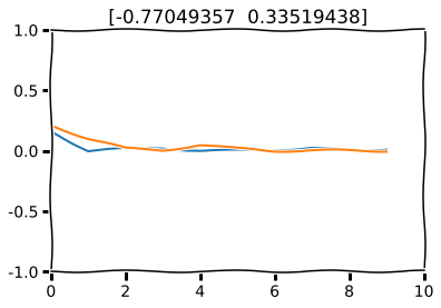
In the next part we will simulate how anomaly detection may work. First let us plot the mean square error of the autoencoder output.
X_test, _ = gen(1)
decoded_imgs = m.predict(X_test)

for i in range(2):
    plt.plot(range(10), np.square(np.abs(X_test[0, :, i] - decoded_imgs[0, :, i])), label="MSE")

plt.ylim(-1,1)
plt.xlim(0,10)
plt.title(dos_numeros)
plt.show()
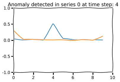
Now let’s change one data point in the generator. This signifies a regime shift.
X_test, _ = gen(1)
X_test[0, 4, 0] = X_test[0, 4, 0] + 0.5
decoded_imgs = m.predict(X_test)

for i in range(2):
    plt.plot(decoded_imgs[0, :, i])
    plt.plot(X_test[0, :, i])

plt.ylim(-1,1)
plt.xlim(0,10)
plt.show()
for i in range(2):
    mse = np.square(np.abs(X_test[0, :, i] - decoded_imgs[0, :, i]))
    anomaly = np.argmax(mse)
    if mse[anomaly] > 0.4:
        plt.title("Anomaly detected in series {} at time step: {}".format(i, anomaly))
    plt.plot(range(10), mse, label="MSE")

plt.ylim(-1,1)
plt.xlim(0,10)
plt.show()
A Note on MSE
Also, assume the financial series is normalized to be a zero-centered signal, MSE would be a mal-adapted measure. Because if the an outlier is near 0, then the MSE will likely be less than the MSE of the original signal(centered at 0). So it is imperative to devise a more sophisticated loss function by adding a moving average to the MSE. This way, we can judge based on the deviations from the rolling average.
A Note on Online Training / Inference
This algorithm, like all signal processing neural networks, should be able to operate on a rolling basis. The algorithm just needs a segment of the data from a sliding window.
When attention mechanism is introduced, online training(input partially observed) becomes more involved. Online and linear-time attention alignment can be achieved with memory mechanism. I might cover attention mechanism for financial data in a future post.
Pattern Search
Given an example trading pattern, quickly identify similar patterns in a multi-dimensional data series.
Implementation:
-
Train a stacked recurrent autoencoder on a dataset of sequences.
-
Encode the query sequence pattern \({\mathcal{X}_{t-1}, \mathcal{X}_{t}, \mathcal{X}_{t+1}, ...}\) to obtain \(H_{\mathcal{X}}\).
-
Then for all historical data, use the encoder to produce fixed length vectors \(\mathcal{H} = \{H_{a}, H_{b}, H_{c}, ...\}\).
-
For each \(t \in \mathcal{H}\), find \(\arg\!\min_t dist(H_{t}, H_{\mathcal{X}})\).
It is basically a fuzzy hash function. This I have not tried since calculating the hash for all sequence requires serious compute only available to big instituional players.

Stacked Autoencoders
This is a good place to introduce how stacked autoencoders work.

As we have seen above, a simple recurrent autoencoder has 3 layers: encoder LSTM layer, hidden layer, and decoder LSTM layer. Stacked autoencoders is constructed by stacking several single-layer autoencoders. The first single-layer autoencoder maps input to the first hidden vector. After training the first autoencoder, we discard the first decoder layer which is then replaced by the second autoencoder, which has a smaller latent vector dimension. Repeat this process and determine the correct depth and size by trial and error(If you know a better way please let me know.) The depth of stacked autoencoders enable feature invariance and allow for more abstractness in extracted features.
A Note on Supervised Learning
This post only covered the unsupervised usage of autoencoders. Variational recurrent autoencoders can “denoise” artifically corrupted data input. I never had any luck with it so I can’t recommend the usage on financial data.
Financial data is extremely noisy. But when trained with a smaller capacity, autoencoders have the built-in ability of denoising because they only learn the most salient features anyway.
A Note on Variational Inference / Bayesian Method
Please refer to this article.
Conclusion
Autoencoders are powerful tools despite their simplistic nature. We use autoencoders to visualize manifold on high dimensional space and detect anomalies in time series.
Reference
https://arxiv.org/pdf/1511.01432.pdf

http://www1.icsi.berkeley.edu/~vinyals/Files/rnn_denoise_2012.pdf

http://www.deeplearningbook.org/contents/autoencoders.html

http://wp.doc.ic.ac.uk/hipeds/wp-content/uploads/sites/78/2017/01/Steven_Hutt_Deep_Networks_Financial.pdf

https://www.cs.cmu.edu/~epxing/Class/10708-17/project-reports/project8.pdf

https://arxiv.org/pdf/1610.09513.pdf

https://arxiv.org/pdf/1012.0349.pdf

https://arxiv.org/pdf/1204.1381.pdf