Backboard Backpropagation: Physical Optimization Using JAX
I came across this video of a basketball back board that is curved in a way so “you can’t miss”. I decided to reproduce this result in 2D using JAX and backpropagation. The idea is very simple: shoot lots of balls, simulate elastic collision, calculate distance from hoop and backpropagate the loss into the board shape. I’m not well versed on phsyical optimization but pretty sure this has been done many times before(BFGS?).
JAX
JAX is a framework developed by Google research that has gained popularity as a much leaner Tensorflow or numpy with autograd. I chose JAX for this project because I can write physics calculations in plain Python as opposed to a DSL. JAX enables forward mode automatic differentiation on Python code across function boundaries including control flow such as for loops and if else.
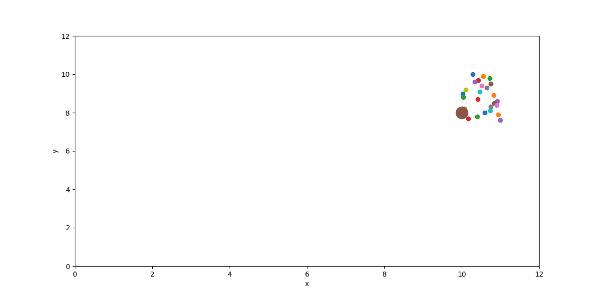
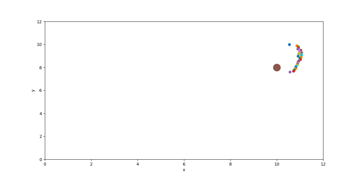
Here is the result:
Before:

After:

Code:
import numpy as onp
import matplotlib.pyplot as plt
import jax.numpy as np
from tqdm import tqdm
from jax import grad, jit, vmap, device_put
from random import uniform

N = 25
H_step = 0.1
H_0 = 10
g = -9.8
hoop_x, hoop_y = (10, 8)

board = device_put(onp.random.rand(N))
# print(board)

@jit
def build_surface(board):
    ret = []
    for i, (a,b) in enumerate(zip(board, board[1:])):
        y_0 = -i*H_step+H_0
        x_0 = a + 10
        y_1 = -(i+1)*H_step+H_0
        x_1 = b + 10
        slope = (y_1 - y_0) / (x_1 - x_0)
        intercept = y_1 - x_1 * slope
        ret.append([slope, intercept])
    return ret

@jit
def solve_t(k, l, x_0, y_0, v_x0, v_y0):
    c = y_0 - k * x_0 - l
    b = v_y0 - k * v_x0
    a = 0.5 * g
    d = (b**2) - (4*a*c)
    sol1 = (-b - np.sqrt(d))/(2*a)
    sol2 = (-b + np.sqrt(d))/(2*a)
    # print(sol1, sol2)
    y_1 = y_0 + v_y0*sol1 + 0.5*g*sol1 ** 2
    y_2 = y_0 + v_y0*sol2 + 0.5*g*sol2 ** 2
    return sol1, sol2, y_1, y_2

@jit
def dist_from_hoop(t, y_f, x_0, v_x0, v_y0):
    x_f = x_0 + v_x0 * t
    v_xf = v_x0
    v_yf = v_y0 + g * t
    cor = 0.81 # https://en.wikipedia.org/wiki/Coefficient_of_restitution
    v_xb = -cor * v_xf
    v_yb = -cor * v_yf

    t = 0.1
    x_b = x_f + v_xb * t
    y_b = y_f + v_yb * t + 0.5*g*t**2
    # print("final_pos", x_b, y_b)
    dist = np.sqrt((x_b - hoop_x)**2 + (y_b - hoop_y)**2)
    return dist

def bounce(board, x_0, y_0, v_x0, v_y0):
    lines = build_surface(board)
    # y_0 + v_y0*t + 0.5*g*t^2 = k(x_0 + v_x0*t) + l
    # (y_0 - k * x_0 - l) + (v_y0 - k * v_x0)*t + 0.5*g*t^2 = 0
    for i, (k, l) in enumerate(lines):
        sol1, sol2, y_1, y_2 = solve_t(k, l, x_0, y_0, v_x0, v_y0)
        t = 0
        y_f = 0
        if sol1 > 0 and -(i+1)*H_step+H_0 < y_1 < -i*H_step+H_0:
            t = sol1
            y_f = y_1
        elif sol2 > 0 and -(i+1)*H_step+H_0 < y_2 < -i*H_step+H_0:
            t = sol2
            y_f = y_2
        else:
            continue

        loss = dist_from_hoop(t, y_f, x_0, v_x0, v_y0)
        return loss
    return 0.

# print(bounce(board, 3.1, 4, 10, 10))

def plot():
    plt.figure(figsize=(12,6))
    # xs = np.arange(8, 12, 0.1);
    # for m, k in build_surface(board):
    #     ys = xs * m + k
    #     plt.plot(xs, ys)
    for i, x in enumerate(board):
        y = -i*H_step+H_0
        print(x+10, y)
        plt.scatter(x+10, y)
    plt.xlim(0, 12)
    plt.ylim(0, 12)
    plt.scatter(hoop_x, hoop_y, s=300)
    plt.xlabel('x')
    plt.ylabel('y')
    # plt.show()


plot()
plt.savefig("orig.png")
for i in tqdm(range(3000)):
    x0 = 0
    y0 = 5
    vx = uniform(7, 10)
    vy = uniform(7, 10)
    board_grad = grad(bounce, 0)(board, x0, y0, vx, vy)
    # print(board_grad)
    board += -board_grad * 0.1
plot()
plt.savefig("optimized.png")